

I work in spreadsheets a lot. It’s still the best way to easily slice and dice small data sets. I’ve been using Google Sheets for most of my spreadsheets for several years, but it has limits. The two biggest are memory and power, and they’ve forced me to keep a few grotesquely large spreadsheets in Excel. Another limitation to Google Sheets that I’ve experienced a lot recently is that you can’t edit row 1 of pivot tables.
When I was learning how to use Google Data Studio I remember the frustration that resulted from trying to connect a Google Sheets pivot table with a Data Studio chart or table. It never worked because the first column of the pivot table was never pulled into Data Studio.
There are forum posts asking about this, with responses saying that it’s not possible. But it’s completely possible. By using a simple spreadsheet hack you can connect a Google Sheets pivot table with Data Studio.
The Problem: A1 is Empty in Google Sheets Pivot Tables
Here’s an example of the problem. Let’s say I have some data in a sheet that looks like this:
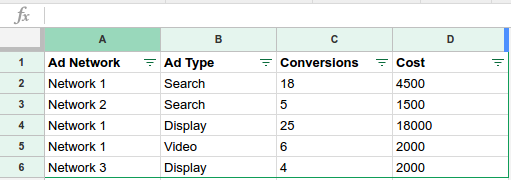
We’ve got some basic ad data: networks, ad type, conversions and cost/spend. Now, assume you want to automatically calculate the cost per conversion of each ad type (column B) and then pull that into Data Studio. That’s a problem because when you create a pivot table in Google Sheets, it doesn’t have a header in column A. This is what the resulting pivot table looks like:
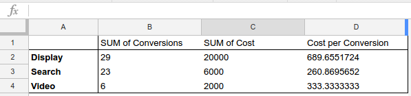
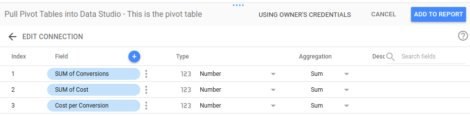
This won’t pull into Data Studio correctly because Data Studio requires a header for every column. If you try to add a pivot table like this to Data Studio, the first column simply won’t show up:
This is unfortunate. Pivot tables are great for slicing and dicing certain types of data. They can help speed up reporting significantly (or even automate it). This simple problem limited me from automating a lot of reports in Data Studio. And then I realized there’s a workaround so easy it’s a bit silly.
The Workaround: Use Formulas to Duplicate the Pivot Table
The solution to this problem is simple:
- Create a new sheet (i.e., tab) in your spreadsheet
- Use formulas to automatically pull over all values from your pivot table
- Replace A1 (and any other headers you want to customize)
- Pull your new sheet (i.e., tab) into Data Studio
I’ve created an example spreadsheet in case anyone is interested in the details. The third tab (where I copy the pivot table) is where the magic happens:
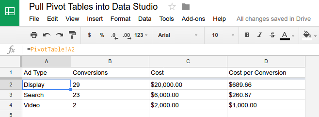
This works as a way to show pivot tables in Data Studio because it allows you to assign a value to A1. Additionally, it allows you to change other column headers. For example, in my pivot table, B1 is “SUM of Conversions,” but in the duplicated sheet it’s simply, “Conversions.” (That’s handy because most pivot table row or column headers can’t be edited in Google Sheets.)
When I create a new tab or sheet like this, I usually do the following:
- Add “-DS” to the end of the sheet name so I know it’s pulling data into Data Studio
- Hide and protect the sheet so that anyone else using the spreadsheet doesn’t view or edit it
This workaround has helped me out quite a bit lately and I hope it helps other people. Feel free to comment below if you have questions or comments.